Visualisation
An Introduction to Statistical Learning
R
It is often convenient to view several plots together.
We can achieve this by using the par() and mfrow() functions, which tell R par() to split the display screen into separate panels so that multiple plots can be viewed simultaneously. For example, par(mfrow = c(2, 2)) divides the plotting region into a 2 × 2 grid of panels.
High-level graphics functions initiate a new plot
curve
svg("curve_sin.svg", width = 11, pointsize = 12, family = "sans")
curve(sin, from = 0, to = 2 * pi, n = 101)
abline(h = 0)
dev.off()

https://www.kaggle.com/learn/intro-to-machine-learning
https://datacarpentry.github.io/R-ecology-lesson/
https://www.stat.cmu.edu/~ryantibs/statcomp/lectures/apply.html
R
- subset
- split
- reorder
- aggregate
- unique
- normalize
- scale
models
All of these take a formula as their first argument, a data frame as their second, subset as their third, weights as their fourth, na.action,…
- lm
- glm
- aov
- loess
- model.matrix
- randomForest (needs to be loaded with library(randomForest))
- lda (needs library(lda))
- naive_bayes (needs library(naivebayes))
- tree (needs to be loaded with library(tree))
- pcr (needs to be loaded with library(pcr)
- plsr
- gam
- gbm
- svm
- survfit
- survdiff
- coxph
- qda
- regsubsets
formula
~ operator
formula = y ~ x1 + x2 + x3
formula = y ~ .
ggplot2
dataframes
Accessing single columns
- Using the dollar sign ($) and the name of the column.
train$Survived - Using square brackets with the index of the column after the comma.
train[,2]
Accessing groups of columns
train[,c("Sex", "Survived", "Age")]train[,c(5, 2, 6)]
dplyr
- Rows
- filter()
- arrange()
- distinct()
- count()
- Columns
- mutate()
- select()
- rename()
- relocate()
- Groups
- group_by()
- summarize()
Predictors
Which predictors are associated with the response?
What is the relationship between the response and each predictor?
Can the relationship between Y and each predictor be adequately summarized using a linear equation, or is the relationship more complicated?
Classifiers
Models
model: an R object, typically returned by ‘lm’ or ‘glm’.
Assessing Model Accuracy
A good classifier is one for which the test error (2.9) is smallest.
Regression Versus Classification Problems
- linear regression
- logistic regression
- Generalized additive models
- boosting
- support vector machines
John Tukey
Tukey introduced the box plot in his 1977 book, “Exploratory Data Analysis”.
He also introduced the word bit as a portmanteau of binary digit and coined the term software.
Python
auto
Auto = read.csv("Auto.csv", header = T, na.strings = "?", stringsAsFactors = T)
advertising
p 121
This is the first linear regression example from Statistical Learning covered in Chapter 2 and 3.
Linear Regression vs K-Nearest Neighbors
7 Questions
- Is there a relationship between sales and advertising budget?
- How strong is the relationship?
- Which media are associated with sales?
- How large is the association between each medium and sales?
- How accurately can we predict future sales?
- Is the relationship linear?
- Is there synergy among the advertising media?
Advertising = read.csv("Advertising.csv", header = T, na.strings = "?", stringsAsFactors = T)
head(Advertising)
  X    TV radio newspaper sales
1 1 230.1  37.8      69.2  22.1
2 2  44.5  39.3      45.1  10.4
3 3  17.2  45.9      69.3   9.3
4 4 151.5  41.3      58.5  18.5
5 5 180.8  10.8      58.4  12.9
6 6   8.7  48.9      75.0   7.2
Advertising = read.csv("Advertising.csv", header = T, na.strings = "?", stringsAsFactors = T)
svg("advertising1.svg", width = 11, pointsize = 12, family = "sans")
plot(sales ~ TV, data = Advertising, col = 2, xlab = "$1000", ylab = "Units Sold")
abline(lm(formula = sales ~ TV, data = Advertising), col = 2)
text(x = 10, y = 7.032594, "7.032594")
points(sales ~ radio, data = Advertising, col = 3)
abline(lm(formula = sales ~ radio, data = Advertising), col = 3)
text(x = 10, y = 9.31164, "9.31164")
points(sales ~ newspaper, data = Advertising, col = 4)
abline(lm(formula = sales ~ newspaper, data = Advertising), col = 4)
text(x = 10, y = 12.35141, "12.35141")
legend("bottomright", legend = c("TV", "Radio", "Newspaper"), fill = c(2,3,4))
dev.off()

iris
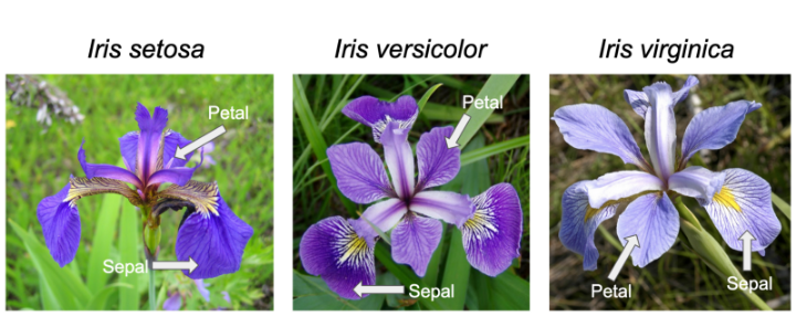
Iris is one of the databases built into R (ie it can be accessed without loading), and used by Learn R through examples among others to teach the basics.
Other built-in datasets include:
- mtcars: Motor Trend Car Road Tests
- ToothGrowth
- PlantGrowth
- USArrests
The data() function provides the full list.
Scatterplot
iris$speciesID <- as.numeric(iris$Species) + 1
iris$shape <- ifelse(iris$Sepal.Length < 5.15, 17, 20)
svg("petal-width-length1.svg", width = 11, pointsize = 12, family = "sans")
plot(Petal.Length ~ Petal.Width, data = iris, col = speciesID, pch = shape)
legend("topleft", levels(iris$Species), fill = 2:4)
dev.off()

dendogram
credit
> Credit = read.csv("Credit.csv", header = T, na.strings = "?", stringsAsFactors = T)
> head(Credit)
   Income Limit Rating Cards Age Education Own Student Married Region Balance
1  14.891  3606    283     2  34        11  No      No     Yes  South     333
2 106.025  6645    483     3  82        15 Yes     Yes     Yes   West     903
3 104.593  7075    514     4  71        11  No      No      No   West     580
4 148.924  9504    681     3  36        11 Yes      No      No   West     964
5  55.882  4897    357     2  68        16  No      No     Yes  South     331
6  80.180  8047    569     4  77        10  No      No      No  South    1151
To get the correlation of “Own”, “Student”, “Married”, and “Region”, these need to be converted to dummy columns with numbers.
house-prices
This is another learning example offered by Kaggle.
The object is to predict SalePrice which is provided in train.csv, but missing in test.csv. The submission should just have two columns, Id and SalePrice.
train <- read.csv("train.csv", header = T, na.strings = "?", stringsAsFactors = T)
ncol(train)
There are 81 columns, so an overhwelming number.
Qualitative Summary
summary(train$MSZoning)
C (all)      FV      RH      RL      RM
     10      65      16    1151     218
summary(train$Id)
“MSSubClass” “MSZoning” “LotFrontage”
[5] “LotArea” “Street” “Alley” “LotShape”
[9] “LandContour” “Utilities” “LotConfig” “LandSlope”
[13] “Neighborhood” “Condition1” “Condition2” “BldgType”
[17] “HouseStyle” “OverallQual” “OverallCond” “YearBuilt”
[21] “YearRemodAdd” “RoofStyle” “RoofMatl” “Exterior1st”
[25] “Exterior2nd” “MasVnrType” “MasVnrArea” “ExterQual”
[29] “ExterCond” “Foundation” “BsmtQual” “BsmtCond”
[33] “BsmtExposure” “BsmtFinType1” “BsmtFinSF1” “BsmtFinType2”
[37] “BsmtFinSF2” “BsmtUnfSF” “TotalBsmtSF” “Heating”
[41] “HeatingQC” “CentralAir” “Electrical” “X1stFlrSF”
[45] “X2ndFlrSF” “LowQualFinSF” “GrLivArea” “BsmtFullBath”
[49] “BsmtHalfBath” “FullBath” “HalfBath” “BedroomAbvGr”
[53] “KitchenAbvGr” “KitchenQual” “TotRmsAbvGrd” “Functional”
[57] “Fireplaces” “FireplaceQu” “GarageType” “GarageYrBlt”
[61] “GarageFinish” “GarageCars” “GarageArea” “GarageQual”
[65] “GarageCond” “PavedDrive” “WoodDeckSF” “OpenPorchSF”
[69] “EnclosedPorch” “X3SsnPorch” “ScreenPorch” “PoolArea”
[73] “PoolQC” “Fence” “MiscFeature” “MiscVal”
[77] “MoSold” “YrSold” “SaleType” “SaleCondition”
[81] “SalePrice”
titanic
Introductory Example
Kaggle provides a training set (which includes the result, Survived, along with various predictors), a test set which doesn’t include Survived, and a simple example gender_submission.csv to show how results should be submitted.
Writing submission file
The model used for gender_submission.csv is all female passengers survived and all male passengers didn’t.
test <- read.csv("test.csv", header = T, na.strings = "?", stringsAsFactors = T)
test$Survived <- as.integer(test$Sex == "female")
write.csv(test[,c("PassengerId","Survived")], "submission.csv", quote = F, row.names = F)
Checking accuracy of “all females lived, all males died” assumption.
train <- read.csv("train.csv", header = T, na.strings = "?", stringsAsFactors = T)
train$Prediction <- as.integer(train$Sex == "female")
(sum(train$Survived == train$Prediction)/nrow(train)) * 100
On the training data, this assumption gives 78.67565% accuracy.
wage
Ordering boxplots
Ordered By Marital Status
Base plot
Wage = read.csv("Wage.csv", header = T, na.strings = "?", stringsAsFactors = T)
new_order <- with(Wage, reorder(maritl , wage, median , na.rm=T))
svg("ordered-maritl.svg", width = 11, pointsize = 12, family = "sans")
plot(new_order, Wage$wage)
dev.off()

ggplot2
library(ggplot2)
Wage = read.csv("Wage.csv", header = T, na.strings = "?", stringsAsFactors = T)
new_order <- with(Wage, reorder(maritl , wage, median , na.rm=T))
svg("ordered-maritl-ggplot2.svg", width = 11, pointsize = 12, family = "sans")
ggplot(data = Wage, mapping = aes(x = new_order, y = wage)) +
  geom_boxplot(fill = c(2, 3, 7, 4, 8), alpha = 0.2) +
  xlab("Marital Status") +
  ylab("Wage")
dev.off()

Finding variable of interest
x must be a numeric vector
d3
geojson
The media type for GeoJSON is “application/geo+json”.
{
    "type": "Feature",
    "properties": {
        "name": "Coors Field",
        "amenity": "Baseball Stadium",
        "popupContent": "This is where the Rockies play!"
    },
    "geometry": {
        "type": "Point",
        "coordinates": [-104.99404, 39.75621]
    }
}
- Geometry
- a region of space
- Feature
- a spatially bounded entity
- FeatureCollection
- a list of Features
{
       "type": "FeatureCollection",
       "features": [{
           "type": "Feature",
           "geometry": {
               "type": "Point",
               "coordinates": [102.0, 0.5]
           },
           "properties": {
               "prop0": "value0"
           }
       }, {
           "type": "Feature",
           "geometry": {
               "type": "LineString",
               "coordinates": [
                   [102.0, 0.0],
                   [103.0, 1.0],
                   [104.0, 0.0],
                   [105.0, 1.0]
               ]
           },
           "properties": {
               "prop0": "value0",
               "prop1": 0.0
           }
       }, {
           "type": "Feature",
           "geometry": {
               "type": "Polygon",
               "coordinates": [
                   [
                       [100.0, 0.0],
                       [101.0, 0.0],
                       [101.0, 1.0],
                       [100.0, 1.0],
                       [100.0, 0.0]
                   ]
               ]
           },
           "properties": {
               "prop0": "value0",
               "prop1": {
                   "this": "that"
               }
           }
       }]
   }
   {
       "type": "MultiLineString",
       "coordinates": [
           [
               [170.0, 45.0], [180.0, 45.0]
           ], [
               [-180.0, 45.0], [-170.0, 45.0]
           ]
       ]
   }
   {
       "type": "Feature",
       "bbox": [-10.0, -10.0, 10.0, 10.0],
       "geometry": {
           "type": "Polygon",
           "coordinates": [
               [
                   [-10.0, -10.0],
                   [10.0, -10.0],
                   [10.0, 10.0],
                   [-10.0, -10.0]
               ]
           ]
       }
       //...
   }